First, let’s build a very simple matrix to help us debug and demonstrate how the calculations are performed when the calculation group is applied:
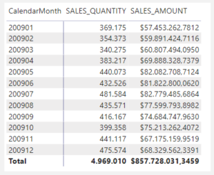
Let’s also create two new measures, one for Sales Month-to-Date (MTD) and another for Sales Year-to-Date (YTD), using the following code:
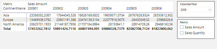
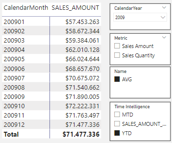
Moving those two new calculations into our matrix and opening the Year-Month column into dates, we can see how these two Time-Intelligence formulas work, the MTD will sum the Sales Amount day by day within a certain month (restarting when a new month starts) while the YTD will sum the Sales amount day by day ignoring the month change:
More about those two Time Intelligence DAX Functions can be found here: Dax Guide.
Assuming that for now you have already installed the Tabular Editor tool and restarted you Power BI Desktop app, from the Top ribbon in Power BI Desktop, let’s launch the Tabular Editor from the External Tool Tab:
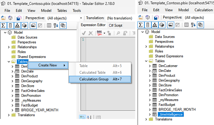
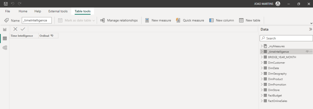
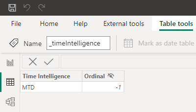
Once Tabular Editor is open, we can expand the “Tables” folder. Then, we can start playing with the Calculation Groups! First, click with the right button of the mouse to open the options for the Tables and then select “New” > “Calculation Group”. Let’s name it “_timeIntelligence”:
You can also rename the “Name” column to something that will be more understandable for you and your users:
At the top ribbon, let’s save and publish the changes to the model.
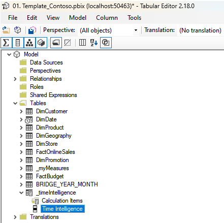
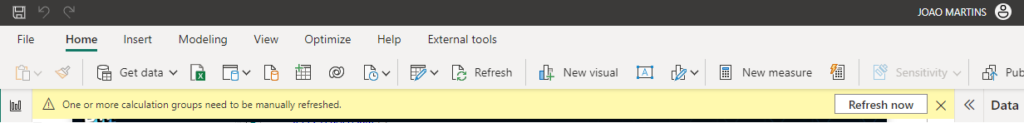
When you go back to the Power BI Desktop file, a warning message at the top will appear, indicating that a Calculation Group has changed and you need to refresh the model in order to see these changes in place. After refreshing the file, you’ll notice that a new table is created on your model, the Calculation Group table.
For now, the table is empty because we haven’t created any Calculation Item yet. But notice that we’ve got a table and a column… A COLUMN! This means that we can use this column to slice and dice our data in our Report! Thus, we can use this column on slicers, matrixes columns or rows or visual axis.
Now, let’s go back into the Tabular Editor app to create our first Calculation Item, the Month-to-Date (MTD) Pattern. To do that, click with the 2nd button of the mouse over the Calculation Group table, select “Create New” > “Calculation Item”:
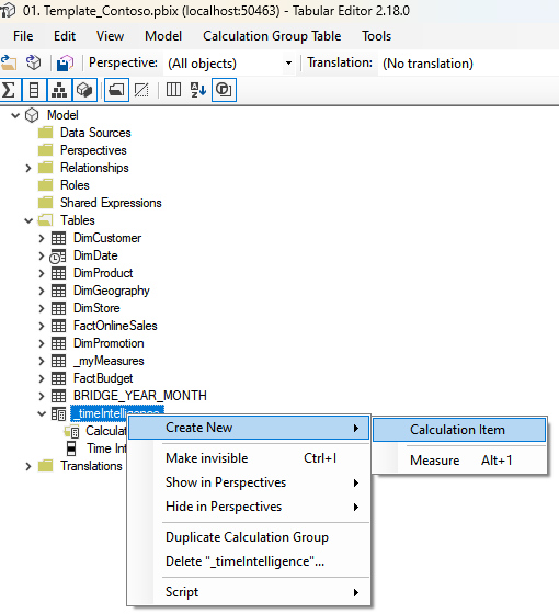
A New Calculation Item will appear on the list below the “Calculation Items” folder. You can rename it as you want. After that, we just need to create the pattern we want:
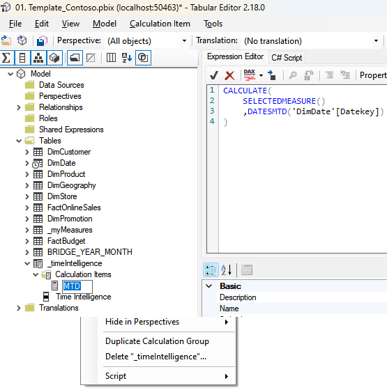
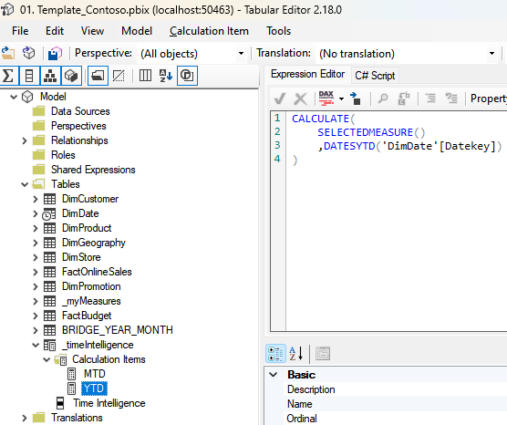
Within the Calculation Item expression, you can place the following code:
Notice here, we’re using a special DAX Function: SELECTEDMEASURE(). This is a restricted function which can only be used within Calculation Items. Basically, when we apply the calculation item, this function will pick up (on the fly during DAX evaluation) the measure that is being used on the visual and will put this measure on the same place where the function is placed within the pattern.
After saving and publishing the Calculation Group to the model, we now can see on the table that a row was created containing the name of our calculation item:
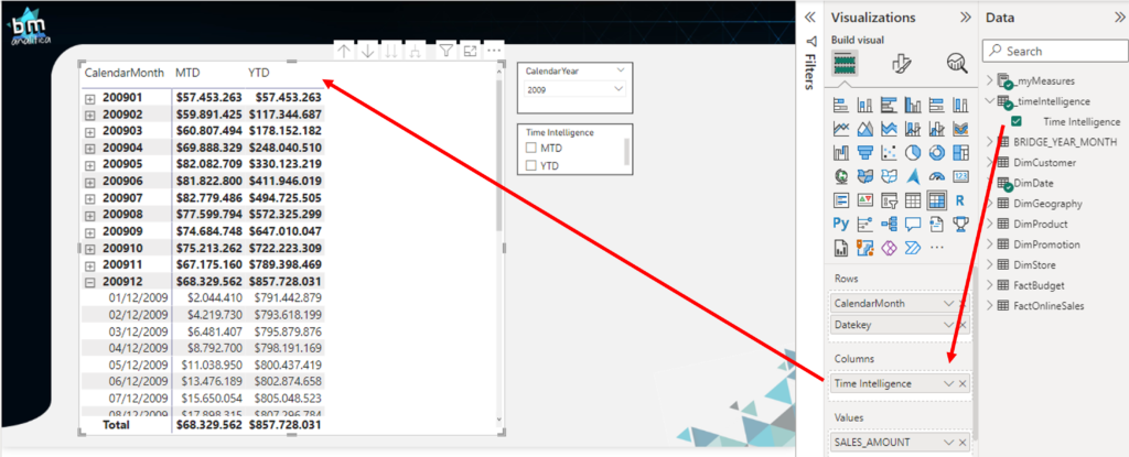
To see the Calculation Group working, let’s go back to our matrix and drop a slicer on the Canvas. In this slicer, let’s drag the Calculation Group column:
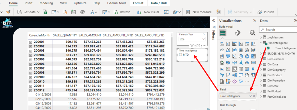
This is when the “MAGIC” begins. Let’s selected on the slicer the MTD item and evaluate the result on the matrix rows (day by day):
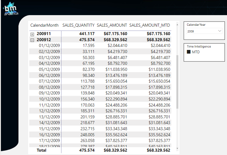
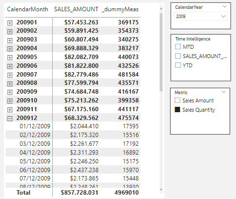
Notice how the numbers for the [SALES_QUANTITY] and [SALES_AMOUNT] are summing up on a Month-to-Date basis (you can compare the [SALES_AMOUNT] with the [SALES_AMOUNT_MTD] formula). For all the measures into the the Matrix, the same pattern MTD pattern was applied!!
Thus, this technique is able to save us a a lot of time and effort when creating any MTD measures, just because we don’t need to create then anymore! We just need to create a “base measure” and then use the Calculation Group in a slicer (or even directly on the matrix columns) to have this pattern applied and the expected output calculated.
Let’s create another Calculation Item. This time, let’s create the Year-to-Date measure:
After saving, publishing and refreshing the Power BI Model, we will see on the Slicer that the new item is there. On the matrix, let’s keep only the [SALES_AMOUNT] measure and place the Calculation Item on the Column field, as showed below:
Notice! Now we’ve got two columns, each containing a different pattern that is being applied to the same base measure!
Let’s add the [QUANTITY_UNITS] measure on our matrix:
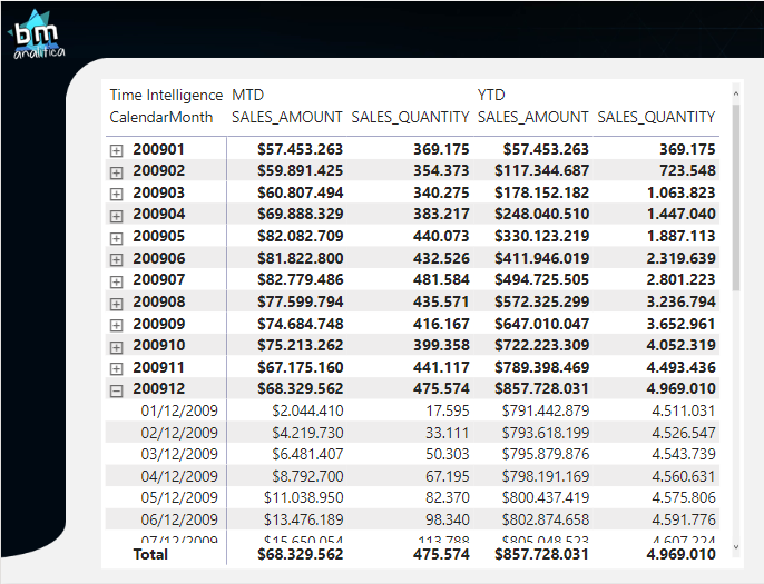
Look carefully! Each pattern is applied to each measure simultaneously without the need of creating more and more measures!!
Well, this is the basic behavior of a Calculation Group. Let’s check now what the calculation item truly does behind the scenes on the next section.
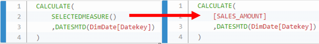
Thus, as you could see, the Calculation Item basically applies its pattern to a measure. However, notice that we had to put inside the pattern the DAX Function SELECTEDMEASURE().
What would happen if we directly include a measure there? Let’s investigate this scenario with the following code:
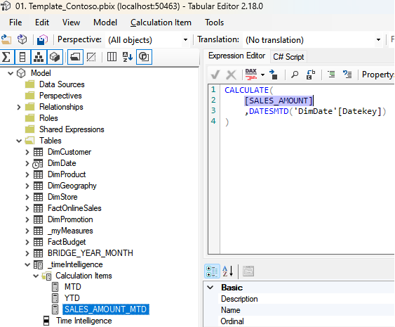
On this code, we removed the SELECTEDMEASURE() formula and put the [SALES_AMOUNT] measure itself. Now, let’s go back to the Power BI Report, keep on our matrix only the [SALES_AMOUNT] and [SALES_QUANTITY] measures and remove the Calculation Group from the matrix columns. Then, let’s select on the slicer the SALES_AMOUNT_MTD item:
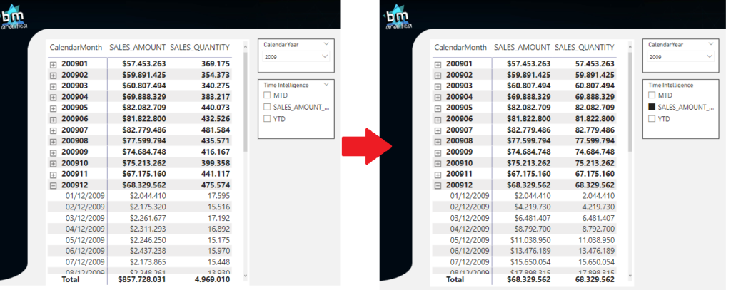
Notice on the right matrix that the numbers are exactly the same for both measures. Thus, what is happening??
Again, the calculation item is a PATTERN. This pattern will be applied (enforced) to whatever measure is placed on your canvas (where the slicer can filter or where you drop the column from the Calculation Group). Once this pattern is “enforcing” the calculation of a specific measure ([SALES_AMOUNT]) and is not anymore adjusted to get the measure over which it is being applied to (SELECTEDMEASURE() ), then basically what the Calculation Item is doing is “stealing” or “replacing” your measure and applying the fixed pattern defined on it.
A very common business scenario to take advantage of this behavior was to use a slicer to select which measure to show on a visual. For example, let’s say we’ve got the following visual containing the [SALES_AMOUNT] measure.
What if, for the same chart, we want to dynamically change the measure on the visual? This means, we want to use a slicer and select what is shown on the visual.
Prior to the existance of Calculation Groups in Power BI, the only way to do this was to use bookmarks to hide/unhide many visuals. Depending on the amount of metrics, this could be a potential issue, for example, if we want to change the Title of the visual, we would need to do that for each hidden visual for each metric (and the chance to forget to do for one of them and receiving the complaint from a user is huge).
In order to deal with this bussines scenario, we can create a new Calculation Group in which for each Calculation Item we’re going to define a 1:1 relation to a measure already built-in the model, like the figure below:
Now, we can place this Calculation Group in a slicer and use it to switch which measure is going to be shown on the visual:
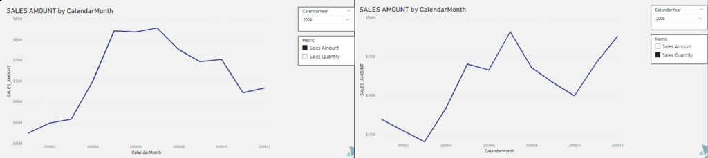
As you can see, on the right, the Sales Amount value keeps the same. However, when on the slicer we select “Sales Quantity” the line changes itself and now it contains the measure itself (notice that Title Name and Axis Name will not change).
We can even use this slicer as a “legend” on the visual. Then, both lines will be shown in the same visual:
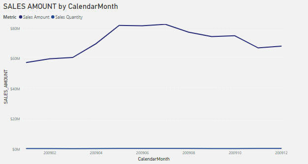
As you can see, this approach will replace any measure which the slicer can affect. Thus, a good practice is to create a “dummy measure” to protect any other measure / visual on the canvas to not be affected by this Calculation Group. To do that, let’s create a dummy measure on our report, like the one below:
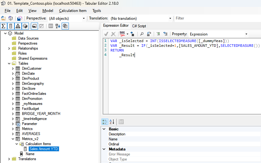
Then, on each Calculation Item for the Metrics we can use the DAX Function ISSELECTEDMEASURE(). Basically, with this function, we’re able to capture the name on which measure the Calculation Item will be applied. Knowing the measure, we’re able to create a protection, like the one below:
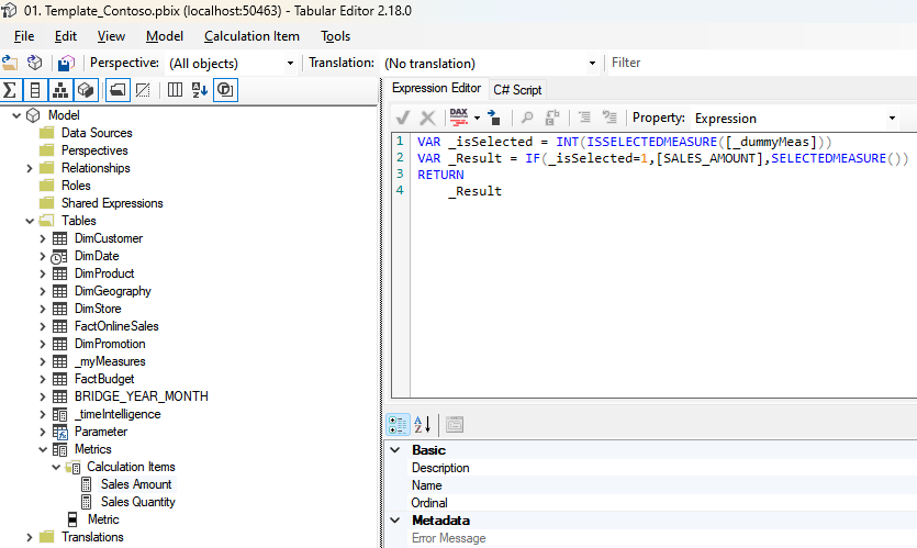
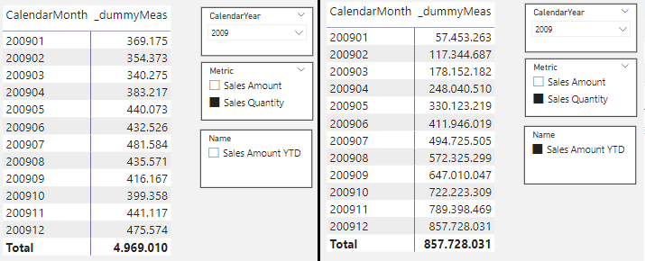
By doing this, the calculation item will be only applied where the [_dummyMeas] is placed.
As you can see on the matrix above, the Calculation Item (“Sales Quantity”) will only affect the column containing the [_dummyMeas] in the matrix, keeping the column with the Sales Amount intact.
This strategy for toggling between measure is already obsolete, once Power BI has launched a new feature called “Field Parameters” that allows the user to choose which measure they want to view in a visual.
However, in some cases, the Calculation Group for measures is still useful. One scenario is to order (drill down and up) on a matrix visual to guarantee the exact order in which the fields are shown. For example, let’s say that our user requires to see in a matrix each measure on a monthly basis:
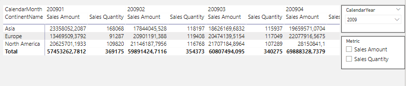
Note that both measures are shown each month. What if we want to see all month for one measure and then all the months to the other measures? Using Field Parameters this is not possible as well as changing this default matrix layout. The only possible way is through Calculation Groups and the drill-down over the columns:
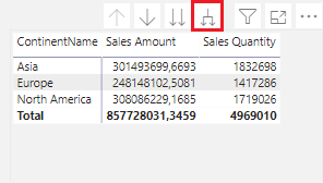
Thus, as you can see, we’re able to burst each measure individually on a Year-Month basis instead of opening both measures within each month.
One of the most important configurations in the Calculation Groups is the Precedence. This only matters when we’ve got more than one Calculation Group in our model, specially if their pattern uses the same dimension table to apply any sort of filter.
Before starting this section, it’s worth to mention that most of it was inspired by this article of SQLBI.
Let’s imagine that we’ve got two Calculation Groups with one calculation item each, Calc Group A and Calc Group B. This configuration will determine, in the moment when a calculation item is applied, which calculation item will be applied first, i.e., when the DAX is will be evaluated and the result computed. This means, if Calc Item from A will be applied and then B or if B will be applied first.
At first sight, one might imagine that this could not generate any problem. However, remember the behavior of the calculation item: it steals the measure and then applies what it has inside it. This changes everything!
For the first example, we’ve just created a new Calculation Group containing a measure reference ([SALES_AMOUNT_YTD]), like the one on the previous section:
Going back to the report, let’s apply first only the first Calculation Group and later both together, as shown on the figure below:
As you can see, on the table in the right, the “Sales Amount YTD” is the Calculation Item that is in fact applied on the matrix. This is because the “Metrics_v2” Calculation Group has a higher Precedence over the “Metrics” one, which means it will be applied first.
Now, let’s build two Calculation Groups, one for Time Intelligence (already created previously in other examples) and another for computing some averages.:
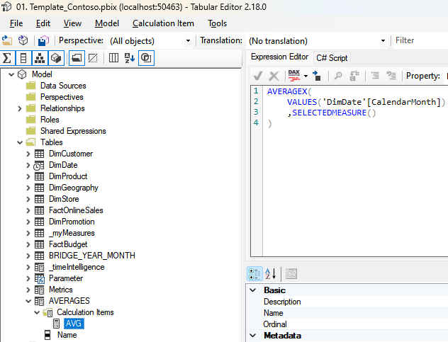
This second Calculation Group is only getting the measure and performing an average over the Date Table. When applying each of the Calculation Groups individually, we’ve got the following result:
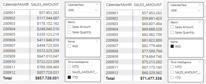
As one could expect, the Average over the month is the month itself, however at the bottom line we’ve got the 857.728.031/12, which is 71.477.336. The YTD is very straightforward.
However, what would happen if we applied both of them simultaneously? Are we going to do an YTD over the Average or are we going to Average the YTD value? Let’s try it:
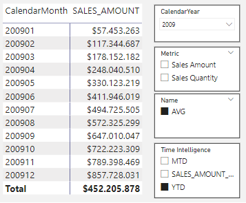
Well, looks like nothing is happening here. But, pay attention at the bottom line. The 452.205.878 is exactly the average of the sum of each row on the table above divided by 12. Remember the behavior of AVG over a monthly basis and that the value on the row didn’t change? The same thing is happening here. Thus, the AVG is being applied over the YTD Calculation.
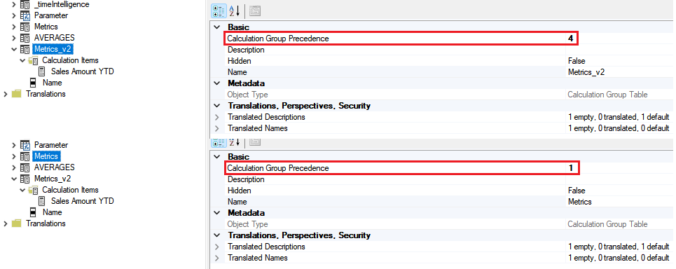
If we investigate the configurantion of each Calculation Group using Tabular Editor and their Precedence, we can notice that:
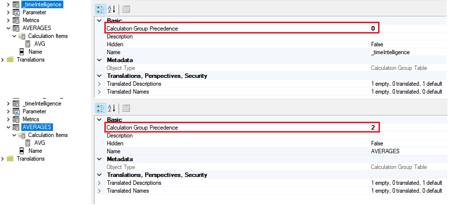
We can notice that the AVERAGES has a higher Precedence than the _timeIntelligence, which means it will be applied first.
Let’s change the Precendence of the _timeIntelligence to 3, higher than the AVERAGES, in order to see how it’s going to behave:
Now, as you can see, the result is very different from the previous one. Notice that now we’re applying the Average and then the YTD. The following excel table can help us debug the result:
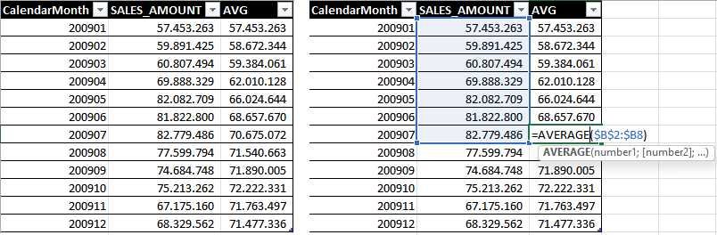
Notice that on the average formula we have frozen the first cell while letting the second to run. In the end, once the YTD Precedence is higher than the AVG, the following DAX code is generated:
[1] https://learn.microsoft.com/en-us/analysis-services/tabular-models/calculation-groups?view=asallproducts-allversions — Documention on Microsoft Learn
[2] https://www.sqlbi.com/articles/introducing-calculation-groups/ — this is the first article from a thread made by SQLBI. All of them are great and are a must read.