Power BI Data Modelling Best Practices

What is Data Modelling?

When working with Analytical tools, we need to import data, usually in the format of tables, into the tool in order to start performing calculations and to display values in any sort of visuals.

The Data Model is the approach we can “connect” those tables by creating relationships between them in a way that the Calculation Engine behind the Analytical tool is able to understand how to relate one table to another to generate the expected result for a calculation. Thus, the Data Model is the combination of Tables, their relationships and the rules to calculate a measure.

The Data Model is an important part (if not the most one) for building accurate, precise, fast and trustable data assets which users can use to unlock impactful insights and drive valuable actions. Having accurate and fast data models is an important part within the implementation of a Data-Driven culture in organizations. This will support users to stop using traditional ways of analyzing data (mainly through Excel spreadsheets), guaranteeing a better productivity for employees (time-wasting preparing those spreadsheets or waiting someone to send the data) and a single source-of-truth for a metric, i.e., unique set of business rules applied to the data to generate a metric (no more excuses that numbers don’t match when different people calculates it – each one with their own and unique set of rules).

Thus, a well-designed data model that guarantees fast performance and accurate numbers is a key component for pavement the road towards a fully data-driven culture within organizations.

Data Models are not just important for Analytical tools, they can also be used in other types of Softwares (like an ERP – SAP/TOTVS/AS400), databases (SQL Server, MySQL, PostgreSQL, Snowflake), Back-end for Apps or even in Data Science projects.

For each tool/application, we have a better design for the data model that will work/perform better. A few examples of data models are:

Big Flat Table (usually created using the main fact against all its dimensions)
Header/Detail (example: customer orders and its lines)
Snowflake (a dimension, connected with another dimension, with another dimension and finally with the fact table)
Star Schema (central fact(s) vs. its dimensions)

Best Data Model Design for Power BI

Being very straightforward, the best model for Power BI (and its VertiPaq Engine) is the Star Schema.

Power BI LOVES the
Star-Schema! A few reasons why:

All the calculations
done by the VertiPaq Engine are highly optimized for this data model (even because data is compressed in a better way in the machine’s memory).
it’s MUCH, MUCH, MUCH easier to write DAX against a Star Schema.
It’s easier to another person understand how the model was built.
Data refresh is faster

The Star Schema is basically defined by two types of data tables: the dimensions and the facts.

How we arrange and connect them is key to have the build the star schema in the right way. First, let’s take a look on how we define each of those types.

Fact Table vs Dimension Table

Prior to start talking about the Star Schema, we must define two main objects used on it: the fact and dimension table.

As the name already propose to us, the Fact Table contains all the facts from the data we want to analyze, i.e., the transactions made by a certain business process. Usually, those facts come together with a timestamp column, like credit card transactions, sales, quantity produced, shipping movements, etc.

The Dimension Table, in the other hand, contains the details/categories of those transactions. An example could be the Product table, which contains name, color, brand. Another one, is the Geography, that contains country, region, city. One curious example of a dimension is the date table, which contains not only the date itself, but also year, month-year, month, month name, etc.

Remember: if the data in a column is aggregated (sum, average, etc.), it could be a fact. If a column is used to slice & dice / categorize data, it could be a dimension (usually, a dimension is what is after the BY clause when one says: “we have to sum this BY …”).

Star-Schema

The Star-Schema, basically, is a data model in which, at the center, we’ve got the Fact Table and around and connected to it we’ve got the Dimension Tables. It’s a middle-term when it regards to normalization/denormalization, it’s not fully denormalized and it’s not fully normalized (once the dimensions could have duplicated values in a column, ex: brand on the product table).

In Power BI, when creating a Star Schema, we’re ALWAYS looking for:

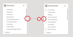
one-to-many relationship, between the Dimension (1-side) and the Fact (many-side).
relationships to be SINGLE-DIRECTION.

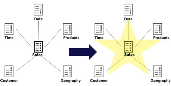
The final goal is to achive a data model that looks like the one below. Achieving a model like this will definitely make your Power BI Journey much easier:

Before ending this section, I would like to make a few remarks:

Avoid at any cost to have MANY-TO-MANY relationships, this WILL degrade the model performance (unless you know VERY VERY well what you’re doing).
Avoid at any cost to use BI-DIRECTIONAL relationships, this will degrade model performance and will generate AMBIGUITY on the model, causing wrong calculations (non-deterministic nature). That are two scenarios which this the bi-directional relationship are allowed to be used: on a bridge table (more details along this article) and at the “leaf” level of a Snowflake Schema (not ideal, but ok).
One-to-One relationshiop could be merged into a single table. If this relationship is only by chance, you should enforce the many side by editing the relationship properties.

Tips & Tricks

Now that your Star Schema is already in place, there are a few more things that you could check to be certain that you have a good model in your hands that can be safely deployed to your users:

Data Integrity

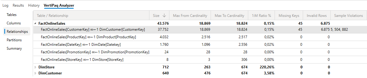
Guarantee that all keys on the Fact Table have their reference on the Dimension Table. Having a key (ex: a brand) in the Fact table which doesn’t have a pair on the Dimension table is considered a Data Integrity issue (that’s why many of the slicers has a “blank” on it. Or the “blank” row in a matrix visual).

You can check the data integrity of your report using DAX Studio.

The Date Table

One of the most important tables in any model.

In order to perform “Time Intelligence” calculations (using DAX functions like DATESMTD(), SAMEPERIODLASTYEAR(), DATESYTD()) we must have a date table on our model which has the day as the table key (i.e., one day per row with no duplicates).

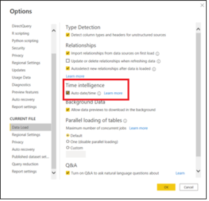
Also, is important to have this table setup correctly and disable the “Auto Date/Time” on the Power BI options. Doing this, you can guarantee that the size of your model is not affected and avoid to use dates from other tables/columns as dimensions on your visuals (thus, avoiding generating wrong values).

In order to disable the “Auto Date/Time”, just go into the Option tab in Power BI and uncheck it from Global > Data Load tab and Current File > Data Load (remember to re-open your PBI file to the effect of the changes):

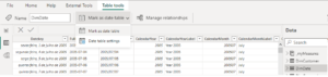
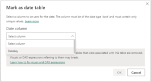
A very important step is, after uploading the Date Table, to mark it as the “Date Table” of the model, thus, the engine will now how to build the query plan when using the Time Intelligence DAX Functions.

fig 7: marking the table as the date table.

fig 8: select the key column from the date table

More about the Date Table, check this article

The "Bridge" Table - and why to bother?

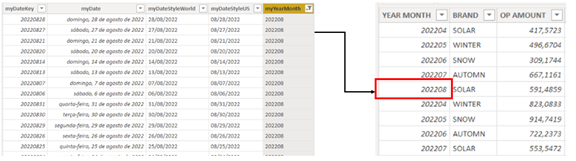
A very common scenario that you might face (if you haven’t already) is to link a dimension table with a fact table when they have different “granularities”, especially if the fact table has a higher granularity than the dimension.

The granularity of a table is the minimum detailed level we can reach in a dimension. For example, on a date table, it would be the date itself. In a time table, it can be the combination of Hour and Minute (17:30) or even just the second.

The complication appears when we’re trying to connect a Dimension Table to a Fact Table, in which the Dimension table is MORE detailed than the Fact Table (example, connect a Date Table that has a daily grain with a budget table containing a year-month grain).

fig 9: connect a daily date table with a year-month budget table

Two very common strategies people are used to do are:

1. A Many-to-Many bidirectional relantionship (which should by HIGHLY avoided)
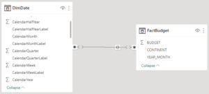
  fig 10: Many-to-Many relationship for tables with different grains
2. Creating a column on the fact table that “tries” to reference the lower grain on the dimension using a Onr-To-Many relationship (mainly applied when we’re working with date granularity)
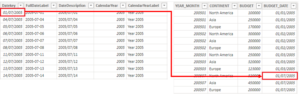
  fig 11: budget table “simulating” a lower grain

Despite of this second option not being the most recommend one, this should not cause big performance issues. It could only generate some hard work to build the DAX Measures.

The best approach to deal with this scenario is to build a “Bridge” (or Factless) table. This table must contain only one column representing exactly the grain level that is common for both tables.

In our example, it is the Year-Month. Then, we build the relationship as following:

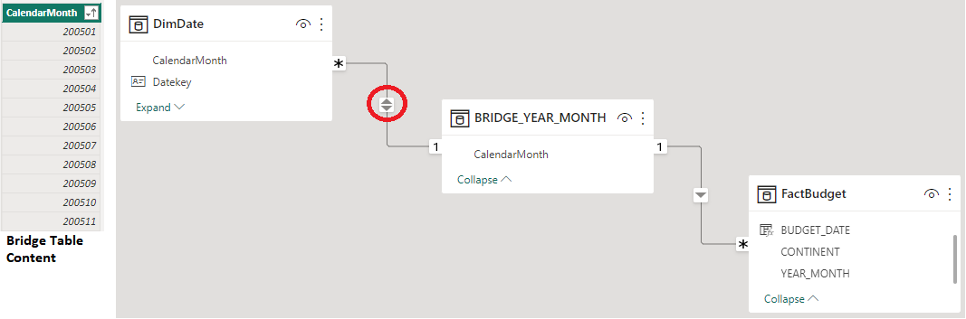
An attention point here is the bi-directional relationship between the DIMENSION table and the BRIDGE. This is the only time in a Power BI Star Schema model that we should use the bi-directional relationship.

The reason for this is very straightforward, we want to propagate the filter on the Date Table up to the higher grain Fact Table. In other words, we want the Date Table to filter the Bridge Table and the bridge to filter the higher grain Fact Table. The only way to do that is enabling the bi-directional filtering.

Despite of this probably causing some performance drawback (once that the bridge and the dimension will have to filter each other, generating more queries than an ideal case of one-to-many relationship), the tables used in this situation are usually small, with a low cardinality, thus, this drawback is not noticed by users.

Avoid Calculated Columns

“Data should be transformed as far upstream as possible, and as far downstream as necessary.” As said by Roche’s Maxim

Try to perform our calculations as close as the source as possible. If we want to join tables that are both in Snowflake, do that there, if we want to join tables that one comes from Snowflake and the other from SQL, use a dataflow. If it’s needed to do a join between some that lives on the dataset with a SQL table, do that on the Power Query.

Only create a calculated column if you need to use a DAX Measure on this column definition.

Date & Time Scenario

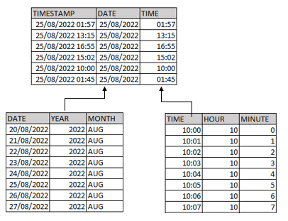
When we’ve got a Fact Table containing a Timestamp, example, a sensor data acquisition, we should break the timestamp into two columns: a date only and a time only.

Then, we should import two dimensions tables, one for Dates and another for Time, creating a one-to-many relationship with the Fact Table:

fig 13: timestamp split into date and time columns

That's all for today folks!

Well well well, this was a very long post, but the idea is to be a guideline that we could review from time to time and not forget any of those good tips. And of course, in future, we could add a few more to this list

I really hope that this article was also useful for you too!

Suggestions? Critics? Questions? Leave a comment below!